The Expectation Maximization Algorithm

The Expectation Maximization (EM) algorithm is a widely used powerful algorithm that can be used to estimate the parameters of a statistical model. It’s similar to the famous Newton-Raphson method, the difference is that the Expectation Maximization (EM) algorithm is used when the data has missing values or when the model has latent variables. It has been applied to a variety of problems, including clustering, density estimation, and parameter estimation for hidden Markov models.

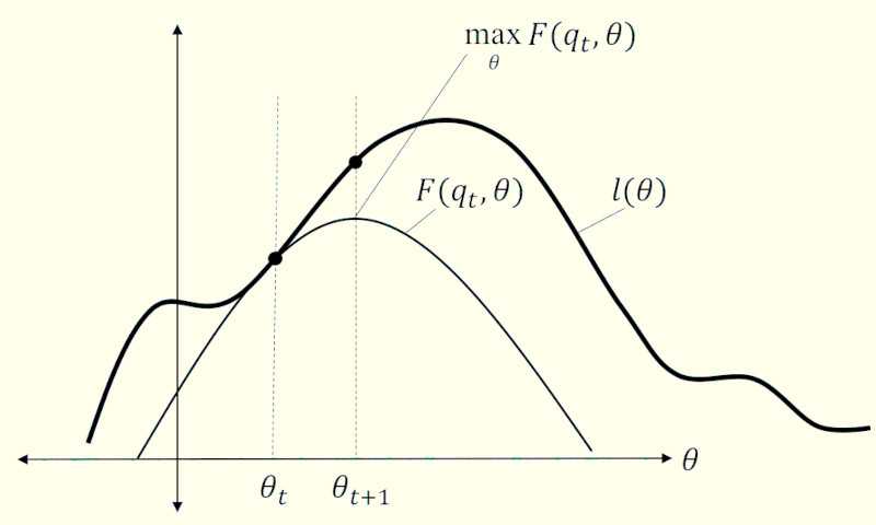
The EM algorithm is an iterative algorithm that consists of two main steps: the E-step and the M-step. In the E-step, the algorithm computes the expected value of the latent variables given the observed data and the current estimate of the parameters. In the M-step, the algorithm maximizes the likelihood function with respect to the parameters, using the expected values of the latent variables computed in the E-step. We repeat these two steps until the algorithm converges to a local maximum of the likelihood function.

Basic Definitions

Convex Set

The Convex Set is defined as a set of points such that the line segment connecting any two points in the set lies entirely within the set. Formally, a set $S$ is a convex set if for any two points $x$ and $y$ in $S$, the line segment connecting $x$ and $y$ lies entirely within $S$.

Convex Function & Concave Function

• Convex Function

The Convex Function is defined on top of the convex set. A twice-differentiable function of a single variable is convex if and only if its second derivative is nonnegative on its entire domain, and its domain should be a convex set. e.g. $f(x)$ is a convex function if $\frac{\mathrm{d^2} f(x)}{\mathrm{d} x^2} \geq 0$ for all $x$ in the domain of $f$.

• Concave Function

The Concave Function is defined on top of the convex set. A twice-differentiable function of a single variable is concave if and only if its second derivative is nonpositive on its entire domain, and its domain should be a convex set. e.g. $f(x)$ is a concave function if $\frac{\mathrm{d^2} f(x)}{\mathrm{d} x^2} \leq 0$ for all $x$ in the domain of $f$.

Jensen’s Inequality

For a convex function $f$ and a random variable $X$, the following inequality holds:

$f(\mathbb{E}[X]) \leq \mathbb{E}[f(X)]$

similarly, but oppositely, for a concave function $f$ and a random variable $X$, the following inequality holds:

$f(\mathbb{E}[X]) \geq \mathbb{E}[f(X)]$

Maximum Likelihood Estimation

In statistics, the Maximum Likelihood Estimation (MLE) is a method used to estimate the parameters of an assumed probability distribution, given some observed data. This is achieved by maximizing a likelihood function so that, under the assumed statistical model, the observed data is most probable. The point in the parameter space that maximizes the likelihood function is called the maximum likelihood estimate. The logic of maximum likelihood is both intuitive and flexible, and as such the method has become a dominant means of statistical inference.

Assuming we have a set of independent and identically distributed (i.i.d.) random variables $X = \{X_{1}, X_{2}, \ldots, X_{n}\}$, and the distribution function is defined as:

$\mathbf{P}(X | \theta) = \prod_{i=1}^{n} P(X_{i} | \theta)$

where $\theta$ is the parameter of the distribution, and we could define the likelihood function as:

$\mathbf{L}(\theta | X) = P(X | \theta) = \prod_{i=1}^{n} P(X_{i} | \theta)$

The Maximum Likelihood Estimation is to find the parameter $\theta$ that maximizes the likelihood function $\mathbf{L}(\theta | X)$, i.e.

$\hat{\theta} = \arg \max_{\theta} \mathbf{L}(\theta | X)$

The Expectation Maximization Algorithm

Definitions

As mentioned before, the Expectation Maximization (EM) algorithm is a loop to iterate between the E-step and the M-step until the algorithm converges to a local maximum of the likelihood function. Let’s say, we have a set of observed data on a random variable $X$, and a latent variable $Z$, and the joint distribution of $X$ and $Z$ is defined as:

$\mathbf{P}(x,z; \theta)$

where $\mathbf{P}$ is the probability mass/density function, $x$ and $z$ are values for $X$ and $Z$, and $\theta$ parameterizes the distribution.

In practice, we often don’t observe the latent variable $Z$, and we wish to find the value for $\theta$ that makes $x$ most likely under our model. Since we have not observed $z$, we take a logarithm of the likelihood function, and the function must marginalize over $z$:

$\mathbf{l}(\theta) = \log \mathbf{L}(\theta | x) = \log \sum_{z} \mathbf{P}(x,z; \theta)$

or,

$\mathbf{l}(\theta) = \log \mathbf{L}(\theta | x) = \log \int \mathbf{P}(x,z; \theta) \mathrm{d}z$

The E-step

The E-step is to compute the expected value of the latent variables given the observed data and the current estimate of the parameters. The expected value of the latent variables is computed using the current estimate of the parameters and the observed data. The E-step is called the “expectation” step because it computes the expected value of the latent variables given the observed data and the current estimate of the parameters.

The M-step

The M-step is to maximize the likelihood function with respect to the parameters, using the expected values of the latent variables computed in the E-step. The M-step is called the “maximization” step because it maximizes the likelihood function with respect to the parameters.

Conclusion

The Expectation Maximization (EM) algorithm is a powerful algorithm that can be used to estimate the parameters of a statistical model. It is a versatile algorithm that can be used in many different settings, and it is an important tool to have in your machine learning toolbox.